
Italiano · English · Français · Deutsch · Русский · Español
In Zurich in 1907 a patient was placed between a battery and a galvanometer, and one watched a spot of light move along a scale. In 1996 a patent automatically corrected the gain of an instrument with two cans and a needle. In between there are eight diagrams. Almost everything changes, except what is being measured.
How to read the diagrams
In every figure a colour always marks the same part, even when its shape changes.
1907: a single loop
The method reaches Jung from Otto Veraguth, a Zurich neurologist, who calls it the “psychogalvanic reflex”. The circuit is as simple as it can be: battery, body and galvanometer in a row. Veraguth states two cells for 2.4 volts and has the subject hold two hollow nickel cylinders, ten centimetres long. The instrument is a mirror galvanometer: a beam of light reflected onto a scale half a metre long. A resistor in parallel with the instrument, the shunt, serves to reduce the swings.
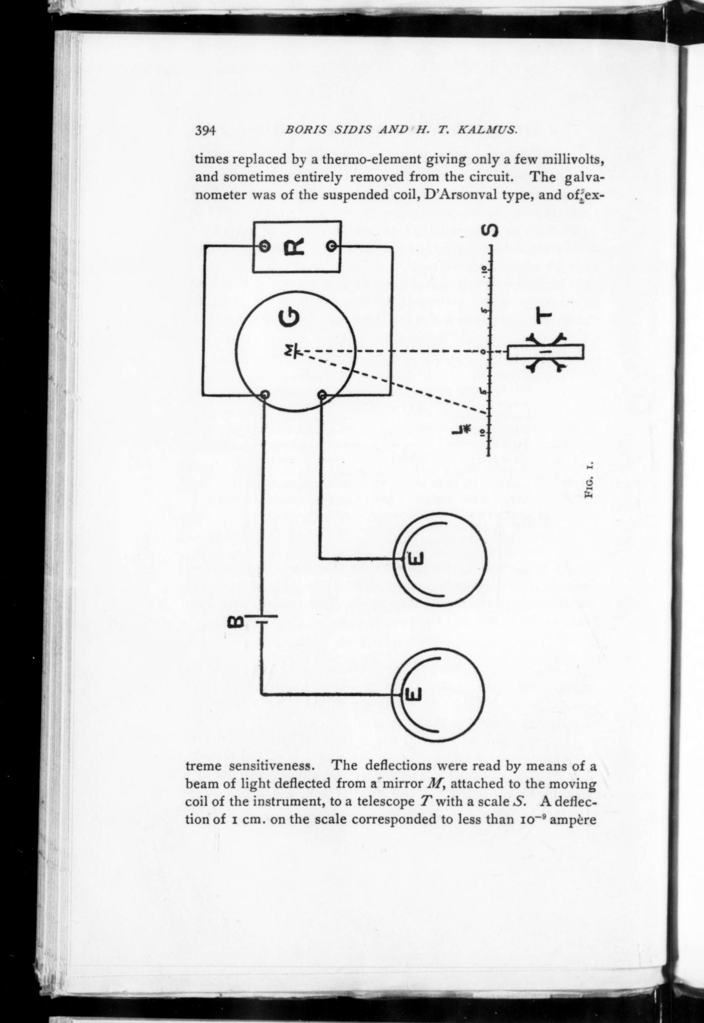
Jung adds a practical idea: a slider that the operator pushes by hand to follow the spot of light, linked to a pen that writes on a roll of paper. He reads a word, waits, watches. The reaction starts one to six seconds after the word. Nobody speaks of resistance in ohms: they count millimetres.
The first figures in ohms come in 1911, from Wells and Forbes, still with the simple loop: a 0.67 volt cell, about 100 microamperes through the body, resistances between 5,000 and 35,000 ohms. Keep these numbers in mind.
1912: the bridge
Gregor and Loewe want to measure the resistance, not just watch it change. They take the circuit used in the laboratory to measure any resistance: the bridge. The body becomes one of the four arms; opposite it goes a known resistance; a slider runs along a wire until no more current flows through the galvanometer. At that point the bridge is balanced, and the position of the slider tells what the body is worth.
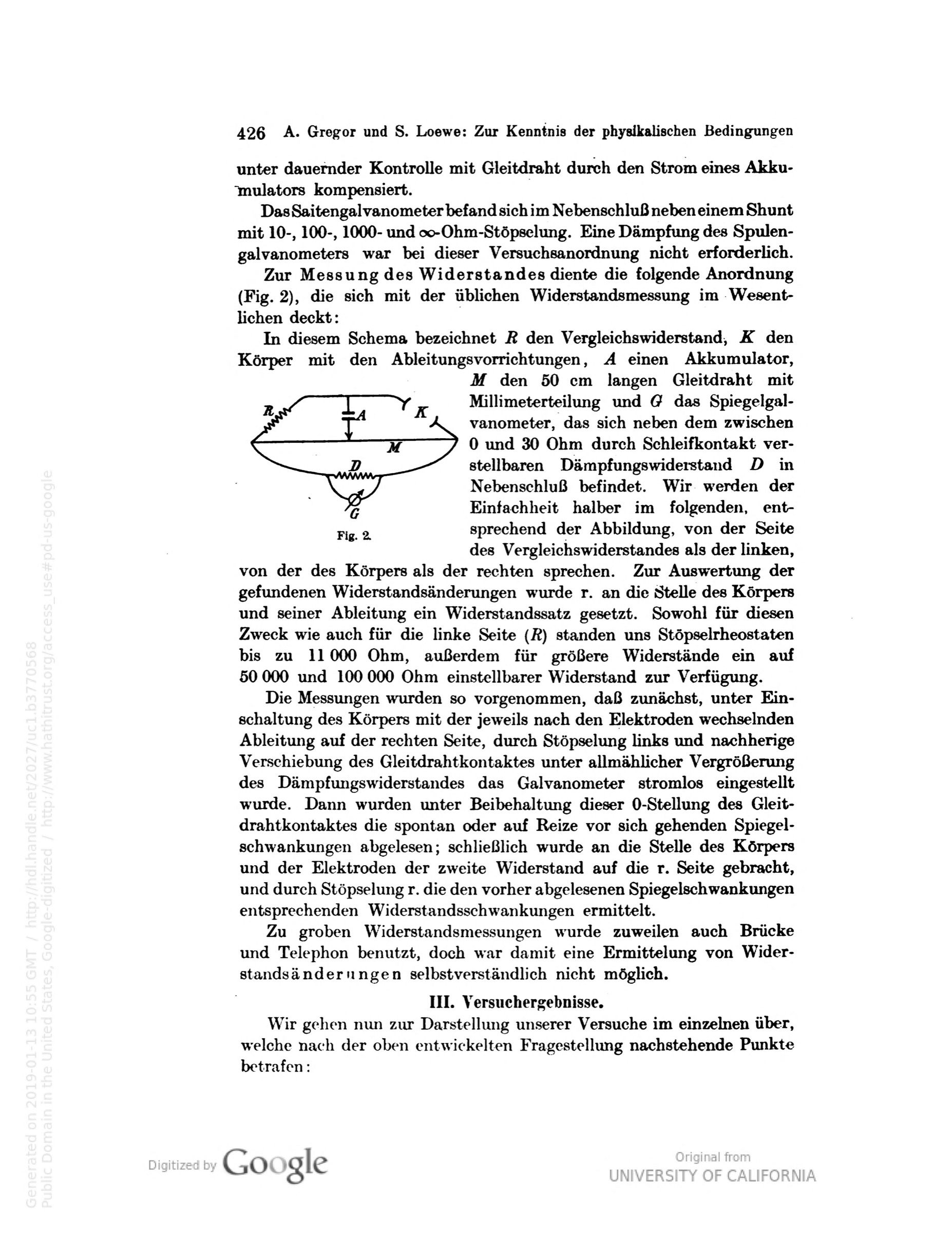
From here on the galvanometer does two jobs. Still at zero, it says that the bridge is balanced and therefore what the resistance is. When it moves, it shows the reaction.
1922: the bridge enters the psychology books
Whately Smith, at Cambridge, publishes The Measurement of Emotion with the complete diagram: a 2 volt cell, two fixed resistors, a resistance box with dials. He balances once at the start and then leaves it alone: he only reads how far the spot of light moves. Three years later David Wechsler publishes a similar circuit, which a Chicago firm puts on sale at 1.5 volts.
1928–1938: the calibrated resistance that brings the needle back to zero
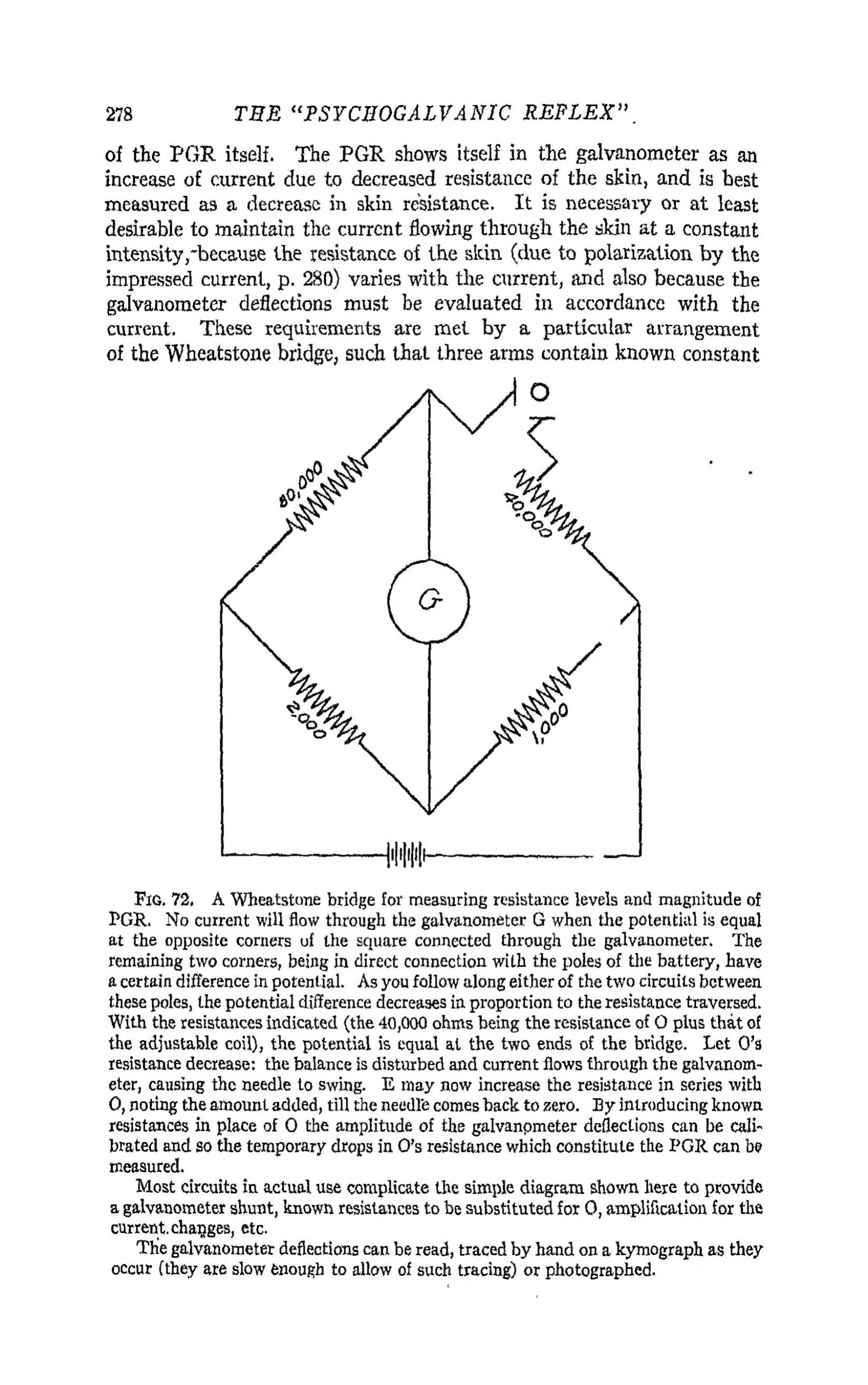
Here is born the gesture that anyone who has used an E-meter knows well. Jeffress, in 1928, puts a resistance box in series with the subject: when the body’s resistance drops, he adds as much again and the needle returns to zero. What he has added is the measurement. Ten years later Woodworth’s textbook, from which generations of American psychologists learned, presents it as the normal circuit:
“Let O’s resistance decrease: the balance is disturbed and current flows through the galvanometer, causing the needle to swing. E may now increase the resistance in series with O, noting the amount added, till the needle comes back to zero.”
— Woodworth, Experimental Psychology, 1938, p. 278.
1928: a valve in place of the galvanometer
The mirror galvanometer is delicate, expensive and needs a dark room. In Sydney, Bellingham, Langford Smith and Martin replace it with a radio valve and a panel needle instrument. They call it the “thermionic bridge”. One turns a potentiometer until the needle sits at mid-scale, then watches:
“…any increase in plate current indicates a decrease in the resistance of the subject, and the deflections are nearly proportional to the alterations in resistance.”
— Australasian Journal of Psychology and Philosophy 6, 1928, p. 140.
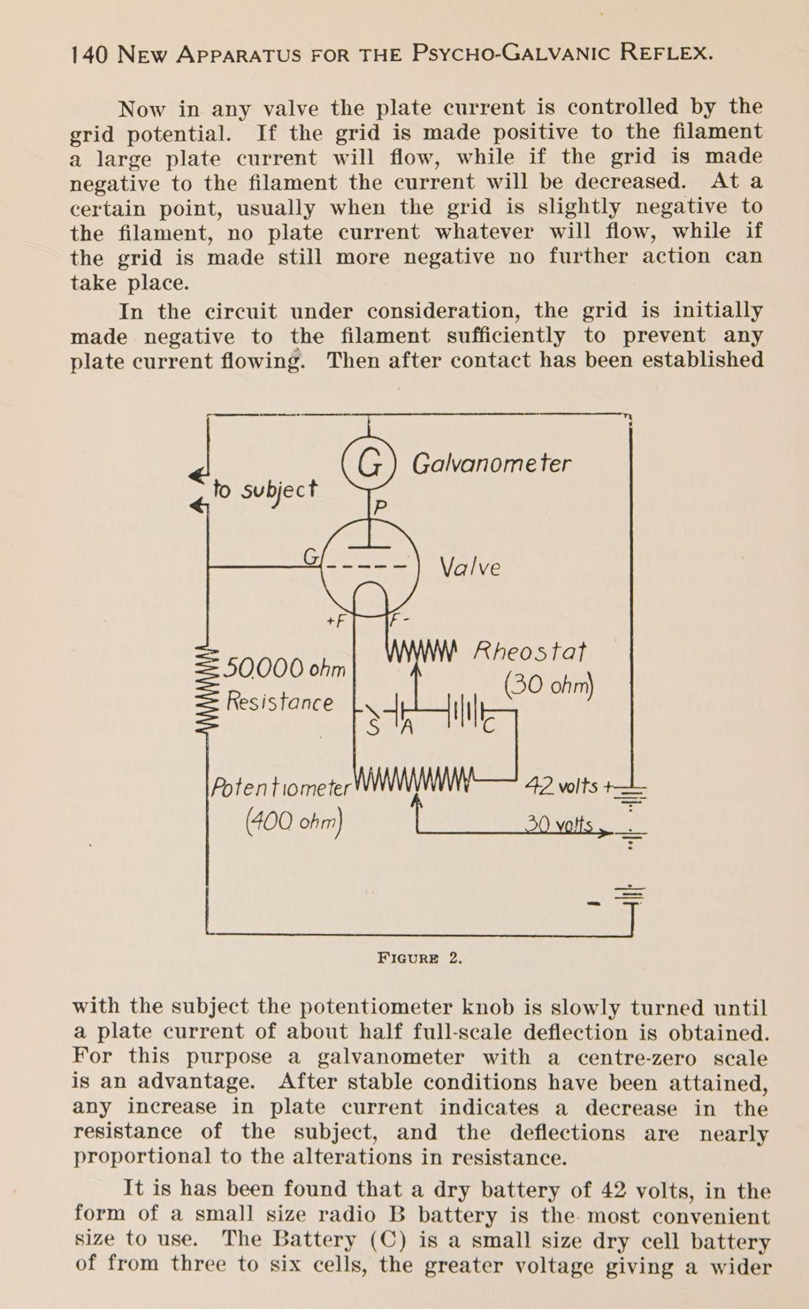
With this all the parts are there: bridge, body on one arm, knob that brings it back to zero, amplifier, panel needle. The year is 1928.
1930: someone points out the flaw
The bridge has a problem, and the psychologists see it at once. The same change in resistance moves the needle more or less depending on the level one is at. R. C. Davis writes it in 1930:
“The most common circuit used for study of the galvanic reaction is the wheatstone bridge… But as it is ordinarily used the electrical relations become extremely complicated, and direct proportionality of deflection to resistance change is lost.”
— Davis, Archives of Psychology 115, 1930, p. 12.
Davis and others respond with constant-current circuits. The bridge, however, remains the standard, flaw and all. Remember it: it comes back at the end.
1951: Mathison
Volney Mathison files his “electropsychometer” on 1 August 1951. In the first line of the patent he states where he starts from:
“It has been known for many years that if a subject is connected in series with a sensitive galvanometer and a source of low-potential direct current […] the psychogalvanometric arrangement as a whole is a valuable adjuvant in psychoanalysis and psychotherapy.”
— US patent 2,684,670.
It is the 1928 circuit inside a box, with a new name on the knob. The electrodes are sponges of metal fabric; the cans arrive shortly afterwards, at someone else’s suggestion.
1966: the Hubbard patent
The patent is titled Device for measuring and indicating changes in resistance of a living body. The valves become three transistors, the supply two batteries, and the knob receives a calibration in ohms: 5,000 ohms at position 2, 12,500 at position 3.
Hubbard himself, in the 1952 manual, does not claim the measurement:
“The measurement of thought with a meter is not new; the understanding and accuracy of measurement is new.”
— Electropsychometric Auditing, 1952.
1996: the flaw of 1930, solved
Davis’s problem remains: with a low tone arm the same reaction makes a big needle movement, with a high tone arm a small one, and the operator has to touch up the sensitivity by hand. US patent 6,011,992, filed in 1996, closes it with a circuit that reads the position of the tone arm and adjusts the gain by itself. The claim says:
“…adjusting the gain of said amplifier circuit according to a predetermined ratio such that a generally constant amplitude response is generated for a measured change in resistance.”
— US patent 6,011,992.
How each part changes
The same thing
Line up the figures stated by the authors, and this is the picture.
| Year | Who | Voltage | Current through the body | Resistance read |
|---|---|---|---|---|
| 1907 | Veraguth | 2.4 V | not given | millimetres only |
| 1911 | Wells and Forbes | 0.67 V | 95–114 µA | 5,000–35,000 Ω |
| 1922 | Whately Smith | 2 V | not given | millimetres only |
| 1925 | Wechsler, commercial version | 1.5 V | not given | read on the bridge |
| 1936 | Ruckmick’s review | — | 40–100 µA | — |
| 1966 | Hubbard patent | 1.5 and 6 V | not given | 5,000 Ω = 2 · 12,500 Ω = 3 |
| 2004 | patent of the digital model | — | no more than 50 µA | in ohms, computed |
One or two cells. A few tens of microamperes from one hand to the other. A skin that is worth between five thousand and a few tens of thousands of ohms, and that for a couple of seconds is worth a little less when something happens to the person. Jung watched it as a spot of light sliding along a celluloid scale; someone using an E-meter watches it as a needle that falls. It is the same physical quantity, measured in the same way, with the same order of current.
What ninety years have added is ease of reading: a way to get back to zero, a number for the level, a sturdy needle in place of a mirror, and in the end a circuit that keeps the amplitude constant.
What is certain and what is not
Read from the original figures and texts: the diagrams of 1908, 1912, 1922, 1928 and 1938; the voltages of Veraguth, Wells and Forbes, Whately Smith; the values in the two patents; all the quotations.
Reconstructed or simplified: the 1907 diagram (Veraguth and Jung describe it only in words); the diagrams of 1951, 1966 and 1996, reduced to the bridge form so that they can be compared.
Second-hand: the voltage of the commercial Wechsler instrument and Ruckmick’s currents come from reviews of 1935–36, not from the original articles.
Not found: a printed diagram by Waller, who nevertheless used the bridge from 1918; Wechsler’s original 1925 article (the figure is known from a 1933 reproduction).